Refactoring - Part II - Porting Over Backtester Logic
Table Of Contents
Recap
Top-Down vs. Bottom-Up
Backtester Design
Porting Calculate pre-cost SR
Fetch Historical Prices
Switching The Data Source
More Duplication
Even More Duplication
Object-oriented programming (OOP)
The Template Class
The Sibling Classes
Back To Top-Level
Recap
In our last article we talked about the importance of refactoring and illustrated the difference between design and implementation by preparing our backtest.py for further refinement. Today we're going to continue to examine our backtesters design and improve its structure by copy-pasting existing code into a more interface focused solution. Our assert() calls will take on the job of protecting us from undesired behaviour changes.
Right now the interfaces we implemented only return literal values. We obviously need to change that. Let's work through them one at a time, starting with the strat_total_perc_returns interface.
def calculate_strat_pre_cost_sr():
return 1.9914208916281093
strat_pre_cost_sr = calculate_strat_pre_cost_sr()
assert (strat_pre_cost_sr == 1.9914208916281093)
It looks like we're testing the end result here. So what's the play? Do we just copy-paste over everything so we get the real result?
Top-Down vs. Bottom-Up
We need to decide on how to approach this. Do we start inside the calculate_strat_pre_cost_sr function and work our way back up? Or should we take a step back and work our way down through the top-level design of our backtester?
Both! Kind of..
When modeling after the fact, it's usually best to use a hybrid approach, switching between the two as the flow of actions dictates. Both have their merits.
The Top-Down approach is more design-driven and focuses on interfaces first. This helps chunking our application into smaller, better manageable components and avoids overfitting our solution to its current state. It's easier to think of what the system ideally should look like when we're not being influenced or limited by past implementation choices.
Bottom-Up on the other hand makes better use of existing code, providing quick feedback, making it faster and easier to iterate.
A hybrid approach then involves using the bottom-up method to refine existing structure while maintaining a top-down perspective to ensure that we're staying true to our overall design. In fact, we already went through this: first we wrote down the top-level design for our backtester and then jumped into some of the deeper nested steps to implement their functions (interfaces). We only did the ones we needed so we can test the assert() calls we had before. We did so by faking the return values inside the functions.
Let's have a look at the top-level design of our backtester again to maintain perspective before we port over its current implementations using bottum-up:
Backtester Design
- Fetch historical price data for instrument to trade
- Configure instrument specs (contract details, trading speed, fee structure, etc.)
- Generate trading signals
- Calculate position size
- Simulate trading
- Calculate pre-cost performance metrics
- Calculate post-cost performance metrics
- Generate performance report
Porting Calculate pre-cost SR
The piece of code we're interested in is this one:
def calculate_strat_pre_cost_sr():
return 1.9914208916281093
How do we migrate its old implementation over into our backtester_refactored.py? This is a function now.. do we copy-paste everything into it? No! Let's quickly take a look at the design of the steps involved for your typical pre-cost SR calculation:
Calculate pre-cost SR Design
- Generate signals (raw forecasts; risk-scaled; rescaled to 10; capped to 20)
- Calculate positions (risk-scaled; incl. rebalancing)
- Calculate strategy raw returns (instr returns * position sizes)
- Calculate pre-cost SR (adjust returns for VOL)
- Annualize pre-cost SR
The top-level design for pre-cost sharpe ratio calculation looks rather simple. We first generate some signals, then calculate desired position sizes based on our risk targeting framework, multiply them with the instruments raw returns to get our raw pnl, which we adjust for volatility to get our daily SR and then annualize it. I've also put some things into parantheses behind each step to allude to deeper nesting inside. If you're not used to thinking in abstracts, you can get lost very quick. The annotations are here to help you keep track of what's happening under the hood to bridge the gap. We'll get rid of them from this part when we go deeper inside the tree.
Let's implement that!
def generate_signals(price_series):
pass
def generate_rebalanced_positions(rebalance_threshold):
pass
def calculate_strat_pre_cost_sr(price_series):
signals = generate_signals(price_series)
rebalanced_positions = generate_rebalanced_positions(rebalance_threshold=10)
raw_usd_pnl = price_series.diff() * rebalanced_positions.shift(1)
pnl_stddev = raw_usd_pnl.ewm(span=35, min_periods=10).std()
raw_returns_vol_adjusted = raw_usd_pnl.mean() / pnl_stddev
return raw_returns_vol_adjusted
# return 1.9914208916281093
strat_pre_cost_sr = calculate_strat_pre_cost_sr(price_series=[])
assert (strat_pre_cost_sr == 1.9914208916281093)
I've abstracted away the more complex logic, namely generate_signals and generate_rebalanced_positions into their own placeholder interfaces. The rest of the logic is pretty straight forward. If we run this, we get all sorts of errors because nothing gets passed in yet. Let's fix that! AttributeError: 'list' object has no attribute 'diff' on price_series.diff() - It looks like we need a price series to kickstart the calculations.
Fetch Historical Prices
**The fetch historical prices design:**
- Fetch raw data for trading frequency from data source
- Clean and prepare data
- Return price series
def fetch_price_series(symbolname, trading_frequency):
from dotenv import load_dotenv
load_dotenv()
# specify data source
import psycopg2
import os
conn = psycopg2.connect(
dbname=os.environ.get("DB_DB"),
user=os.environ.get("DB_USER"),
password=os.environ.get("DB_PW"),
host=os.environ.get("DB_HOST"),
port=os.environ.get("DB_PORT")
)
# fetch from data source
cur = conn.cursor()
cur.execute(f"""
SELECT ohlcv.time_close, ohlcv.close
FROM ohlcv
JOIN coins ON ohlcv.coin_id = coins.id
WHERE coins.symbol = '{symbolname}'
ORDER BY ohlcv.time_close ASC;
""")
rows = cur.fetchall()
cur.close()
conn.close()
import pandas as pd
# "clean" and prepare
df = pd.DataFrame(rows, columns=['time_close', 'close'])
df['time_close'] = pd.to_datetime(df['time_close'])
if not pd.api.types.is_datetime64_any_dtype(df['time_close']):
df['time_close'] = pd.to_datetime(df['time_close'])
df.set_index('time_close', inplace=True)
df.sort_values(by='time_close', inplace=True)
return df.resample(trading_frequency).last()
price_series = fetch_price_series('BTC', '1D')
Great, that bit seems to be working. We run into another error now - AttributeError: 'NoneType' object has no attribute 'shift' on rebalanced_positions.shift(1). Before we fix that, let's pause for a minute.
I think we can build in some more useful assert() calls. In the back of our head looms the very abstract description of fetching historical prices, which doesn't really specify how we should fetch it. If we want to switch out the data source, we don't care about the SQL code anymore. What we DO care about is the structure of the data returned. I'm going to use a little different assert syntax here to show you an option that can be even more verbose.
import pandas as pd
trading_frequency = '1D'
symbolname = 'BTC'
price_series = fetch_price_series(symbolname, trading_frequency)
# Basic DataFrame structure checks
assert not price_series.empty, "DataFrame should not be empty"
assert price_series.index.name == 'time_close', "Index should be named 'time_close'"
assert 'close' in price_series.columns, "DataFrame should have 'close' column"
# Check index properties
assert pd.api.types.is_datetime64_dtype(price_series.index), "Index should be datetime64"
assert price_series.index.is_monotonic_increasing, "Index should be sorted ascending"
# Check for duplicates
assert not price_series.index.duplicated().any(), "Should not have duplicate timestamps"
# Check resampling to trading frequency
time_diffs = price_series.index.to_series().diff()[1:] # Skip first NaN diff
expected_timedelta = pd.Timedelta(trading_frequency)
assert time_diffs.max() <= expected_timedelta, f"Data should be sampled at {trading_frequency} frequency"
# Basic price sanity checks
assert price_series['close'].dtype == float, "Close prices should be float type"
assert (price_series['close'] > 0).all(), "All prices should be positive"
assert not price_series['close'].isnull().any(), "Should not have NaN prices"
# Check reasonable date range
current_year = pd.Timestamp.now().year
assert price_series.index.max().year <= current_year, "Data should not be from the future"
This blob of assert calls does a bunch of checks that are (currently) necessary for our application to work. We can get rid of some of them - like checking for close and time_close as column names - when we refactor to more general interfaces.
Switching The Data Source
Let's put our test suite to work! What if we wanted to use prices from a .csv file instead? We can use our old .csv file from one of the first issues in this series to implement this:
def fetch_price_series(symbolname, trading_frequency):
import pandas as pd
df = pd.read_csv(f'./{symbolname}.csv')
df['time_close'] = pd.to_datetime(df['time_close'])
if not pd.api.types.is_datetime64_any_dtype(df['time_close']):
df['time_close'] = pd.to_datetime(df['time_close'])
df.set_index('time_close', inplace=True)
return df.resample(trading_frequency).last()
If we run this, unfortunately we get an error: KeyError: 'time_close'. That's because the .csv has different column names than the data returned from our database. It looks like we need to be able to tell the interface about it. We need to do the same for the close_price column.
def fetch_price_series_csv(
symbolname,
trading_frequency,
index_column,
price_column):
df = pd.read_csv(f'./{symbolname}.csv')
df['close'] = df[price_column]
df[index_column] = pd.to_datetime(df[index_column]).dt.tz_localize(None)
df.set_index(index_column, inplace=True)
df.sort_values(index_column, inplace=True)
return df.resample(trading_frequency).last()
trading_frequency = '1D'
symbolname = 'BTC'
# coingecko csv format
index_column = 'timestamp'
price_column = 'price'
price_series = fetch_price_series_csv(
symbolname,
trading_frequency,
index_column,
price_column
)
assert price_series.index.name == index_column, f"Index should be named {index_column}"
However, if we run this, we get an error AssertionError: All prices should be positive. Let's investigate that further
print("\nChecking for non-positive prices...")
problematic_prices = price_series[~(price_series['close'] > 0)]
if not problematic_prices.empty:
print("\nFound these non-positive prices:")
print(problematic_prices[['close']].to_string())
print(f"\nTotal problematic prices: {len(problematic_prices)}")
assert not price_series['close'].isnull().any(), "Should not have NaN prices"
assert (price_series['close'] > 0).all(), "All prices should be positive"
# Checking for non-positive prices...
# Found these non-positive prices:
# close
# timestamp
# 2013-06-04 NaN
# 2015-01-28 NaN
# Total problematic prices: 2
# Traceback (most recent call last):
# [...]
# assert not price_series['close'].isnull().any(), "Should not have NaN prices"
# AssertionError: Should not have NaN prices
Weirdly there are 2 NaNs in our price_series. We're going to just fill them for now.
def fetch_price_series_csv(
symbolname,
trading_frequency,
index_name,
price_name):
df = pd.read_csv(f'./{symbolname}.csv')
df['close'] = df[price_name]
df[index_name] = pd.to_datetime(df[index_name]).dt.tz_localize(None)
df.set_index(index_name, inplace=True)
df.sort_values(index_name, inplace=True)
# Resample and handle missing values
resampled = df.resample(trading_frequency).last()
resampled['close'] = resampled['close'].ffill() # Forward fill NaN values
# Print diagnostic info
nan_after_fill = resampled['close'].isna().sum()
if nan_after_fill > 0:
print(f"\nWarning: Still found {nan_after_fill} NaN values after forward filling")
print("First and last dates with NaN:")
print(resampled[resampled['close'].isna()].index[[0, -1]])
return resampled
Even though the .csv file is even more outdated than our database, we now don't get any errors. The structure of what we're reading seems to be fine. Using our new, second datasource doesn't break our application! Later on we're going to add a test that checks if the close price of now - t1 - in our example yesterday - is in there. For this we need more up to date data. We'll come to that soon.
We now face a different problem though. A developers all time classic: duplicated code! Duplication comes in all sorts of forms and we even face multiple different kinds of duplication here. The first one is pretty obvious. It is when the code is literally duplicated letter for letter. Both, the read from csv datasource and the sql reader are loading their data into a dataframe for further juggling before returning the resampled version:
df[index_name] = pd.to_datetime(df[index_name])
if not pd.api.types.is_datetime64_any_dtype(df[index_name]):
df[index_name] = pd.to_datetime(df[index_name])
df.set_index(index_name, inplace=True)
df.sort_values(index_name, inplace=True)
return df.resample(trading_frequency).last()
Duplication can quickly become a nightmare. If for some reason you need to change the logic for cleaning and rearranging your data, with duplicated code you need to fix it in multiple places! Not only does this increase your workload but it'll also be hard to remember all the implementations flying around your code base where you have to change it. In fact, we just now fixed an issue with missing data in the csv reader but not in the db reader. You'll almost always be better of by getting rid of duplication! If two expressions are the exact same, we can simply extract the logic into its own function and call that function instead:
# The extracted logic, previously duplicated
def prepare_price_series(price_series, trading_frequency, index_column):
# Set index
price_series['time_close'] = pd.to_datetime(price_series[index_column]).dt.tz_localize(None)
price_series.set_index('time_close', inplace=True)
price_series.sort_values(by='time_close', inplace=True)
# Resample and handle missing values
resampled = price_series.resample(trading_frequency).last()
resampled['close'] = resampled['close'].ffill() # Forward fill NaN values
# Print diagnostic info
nan_after_fill = resampled['close'].isna().sum()
if nan_after_fill > 0:
print(f"\nWarning: Still found {nan_after_fill} NaN values after forward filling")
print("First and last dates with NaN:")
print(resampled[resampled['close'].isna()].index[[0, -1]])
return resampled
def fetch_price_series_db(
symbolname,
trading_frequency,
index_column,
price_column):
[...]
df = pd.DataFrame(rows, columns=[index_column, price_column])
# calling the extracted logic, passing on arguments
return prepare_price_series(df, trading_frequency, index_column)
def fetch_price_series_csv(
symbolname,
trading_frequency,
index_column,
price_column):
df = pd.read_csv(f'./{symbolname}.csv')
df['close'] = df[price_column]
# calling the extracted logic, passing on arguments
return prepare_price_series(df, trading_frequency, index_column)
trading_frequency = '1D'
symbolname = 'BTC'
index_column = 'time_close'
price_column = 'close'
price_series = fetch_price_series_db(
symbolname,
trading_frequency,
index_column,
price_column
)
# coingecko csv format
index_column = 'timestamp'
price_column = 'price'
price_series = fetch_price_series_csv(
symbolname,
trading_frequency,
index_column,
price_column
)
# Basic DataFrame structure checks
assert price_series.index.name == index_name, f"Index should be named {index_name}"
We now have a centralized prepare_price_series function in which we handle the data cleaning. If we want to change that logic or add to it, we only have one place we need to edit.
Note that after each change, we run our code again to check if we get the same output as before. If at any point we get a different result in our terminal, we need to circle back and inspect the issue further.
More Duplication
The second type of duplication is not so obvious but still obvious to the trained eye. When the code is similar but not exactly the same, we should first seperate the similar bits from the different ones before then handling the rest. Luckily, with our previous extraction we already laid out the groundwork.
The next step kind of depends on what code exactly you're looking at. If you're looking at multiple code pieces doing the same thing but with different algorithms, you should replace one of them with the better algorithm of these two. If that makes your tests fail, you can use the old (replaced) one for debugging. If you look closely, we can see that both price fetching functions also do something with the price column:
def fetch_price_series_db([...])
[...]
df = pd.DataFrame(rows, columns=[index_column, price_column])
[...]
def fetch_price_series_csv([...]):
[...]
df['close'] = df[price_column]
[...]
This fits the description of "using a different algorithm". Both rename the columns to something we specified. Our application is working with a dataframe that has the columns time_close and close. If you print the data returned from our SQL query, we can see that the columns are just named [0] and [1].
0 1
0 2010-07-14 23:59:59 0.056402
1 2010-07-15 23:59:59 0.057568
2 2010-07-16 23:59:59 0.066492
3 2010-07-17 23:59:59 0.065993
4 2010-07-18 23:59:59 0.078814
... ... ...
5349 2025-03-06 23:59:59 89961.727244
5350 2025-03-07 23:59:59 86742.675624
5351 2025-03-08 23:59:59 86154.593210
5352 2025-03-09 23:59:59 80601.041311
5353 2025-03-10 23:59:59 78532.001808
fetch_price_series_db renames these using columns=[index_column, price_colum]. The fetch_price_series_csv also renames the price column, which is named price in the .csv file, to close. So which one is the better algorithm? I'd say neither to be honest.
Let's have a look at a different solution:
def transform_columns(df, index_column, price_column):
column_mapping = {
index_column: 'time_close',
price_column: 'close'
}
df.rename(columns=column_mapping, inplace=True)
return df
# The extracted logic, previously duplicated
def prepare_price_series(price_series, trading_frequency, index_column, price_column):
price_series = transform_columns(price_series, index_column, price_column)
# Set index
[...]
def fetch_price_series_db([...]):
[...]
df = pd.DataFrame(rows)
# Calling the extracted logic, passing on arguments
return prepare_price_series(df, trading_frequency, index_column, price_column)
def fetch_price_series_csv([...]):
df = pd.read_csv(f'./{symbolname}_{trading_frequency}.csv')
# Calling the extracted logic, passing on arguments
return prepare_price_series(df, trading_frequency, index_column, price_column)
index_column = 0
price_column = 1
price_series = fetch_price_series_db(
symbolname,
trading_frequency,
index_column,
price_column
)
index_column = 'timestamp'
price_column = 'price'
price_series = fetch_price_series_csv(
symbolname,
trading_frequency,
index_column,
price_column
)
This algorithm now takes the arguments index_column and price_column and translates them to 'time_close' and 'close' using a mapping dictionary defined in transform_columns.
For the SQL reader the column names passed in are 0 and 1 as previously stated. The CSV version takes the strings 'timestamp' and 'price' and translates them. We embedded that logic into prepare_price_series so everytime we want to "clean" our data, we're renaming accordingly.
A little disclaimer right here: we kind of introduced other issues like tight coupling by hastily copy-pasting things around. We have to deal with this in some kind of way. Hunting down a parameterlist that gets passed around the inheritance tree or trying to figure out where state gets changed is never fun. We'll come to that in a minute, it's a process!
Even More Duplication
Another type of duplication is the case where you're looking at two code pieces that are performing similar steps in the same order but the steps differ in implementation. In this case it's usually better to form a more generalized template out of them and rely on its interface instead. This is the problem we're facing here!
Read from DB design:
- Read data from DB
- Prepare data
- Return data
Read from .csv design:
- Read data from .csv
- Prepare data
- Return data
A more generalized design would look like:
- Read data from datasource
- Prepare data
- Return data
Or in pseudocode:
def fetch_price_series(symbolname, trading_frequency):
price_series = data_source.fetch_price_series(symbolname, trading_frequency)
return prepared_price_series(price_series)
Object-oriented programming (OOP)
We're getting into the realms of object-oriented programming (OOP) now. OOP terms like Inheritance, Polymorphism, SOLID principles etc. often sound very complicated but in my opinion are really just fancy terms for grouping similar properties and behaviour into structured pieces of code to make them easier to work with. Classes are used to group things and objects are just instances of classes.
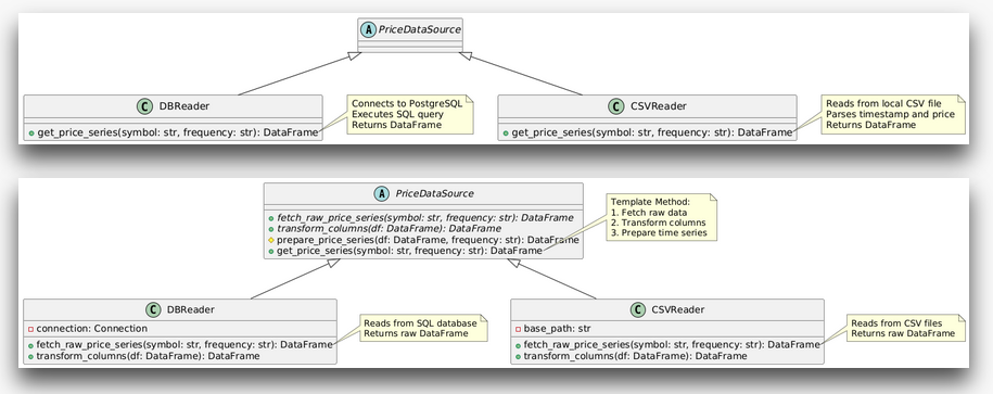
To make this more concrete, let's have a look at an UML diagram of the template design we just talked about. First, the current, duplicated code version.

Both, DBReader and CSVReader are classes with the same interface get_price_series(). They are grouped into the same "type of class", a PriceDataSource because they share the responsibility of providing us with price data. The current implementations of this interface perform the same thing but differ slightly.
Let's now have a look at the improved template version:

In this version the PriceDataSource parent class dictates the general structure of what a data reader should be able to perform. It defines the fetch_raw_price_series and transform_columns as necessary interfaces to be implemented for any class that wants to become a data source. The letter for letter duplications prepare_price_series and get_price_series were extracted and "pulled up" into the parent class. There's only one place we need to look at if we want to debug that logic, the parent class.
Each subclass, namely DBReader and CSVReader inherit the generalized behaviour prepare_price_series and get_price_series. They do not have to define these intefaces themselves anymore since we got rid of their duplication. The only thing they really need to define is the way they connect to their underlying data store and how to translate it into the structure we need for further computation.
If you don't get it yet, that's fine. For some people it's easier to look at code instead. Let's talk about the similar, extracted parts first:
The Template Class
import pandas as pd
from abc import ABC, abstractmethod
class PriceDataSource(ABC):
TARGET_INDEX_COLUMN_NAME = 'time_close'
TARGET_PRICE_COLUMN_NAME = 'close'
def __init__(self, index_column, price_column):
self.index_column_name = index_column
self.price_column_name = price_column
@abstractmethod
def fetch_raw_price_series(self, symbol, frequency):
pass
def transform_columns(self, df):
column_mapping = {
self.index_column_name: self.TARGET_INDEX_COLUMN_NAME,
self.price_column_name: self.TARGET_PRICE_COLUMN_NAME
}
return df.rename(columns=column_mapping)
def prepare_price_series(self, df, frequency):
df = self.transform_columns(df)
df[self.TARGET_INDEX_COLUMN_NAME] = pd.to_datetime(df[self.TARGET_INDEX_COLUMN_NAME]).dt.tz_localize(None)
df.set_index(self.TARGET_INDEX_COLUMN_NAME, inplace=True)
df.sort_index(inplace=True)
# Resample and handle missing values
resampled = df.resample(frequency).last()
resampled[self.TARGET_PRICE_COLUMN_NAME] = resampled[self.TARGET_PRICE_COLUMN_NAME].ffill()
# Print diagnostic NaN info
nan_after_fill = resampled[self.TARGET_PRICE_COLUMN_NAME].isna().sum()
if nan_after_fill > 0:
print(f"\nWarning: Still found {nan_after_fill} NaN values after forward filling")
print("First and last dates with NaN:")
print(resampled[resampled[self.TARGET_PRICE_COLUMN_NAME].isna()].index[[0, -1]])
return resampled
def fetch_price_series(self, symbol, frequency):
raw_df = self.fetch_raw_price_series(symbol, frequency)
return self.prepare_price_series(raw_df, frequency)
The parent class PriceDataSource now holds all the logic that is similar across sibling classes. It takes care of the general flow of logic fetch_price_series which is taking care of fetching raw data and then preparing it for further processing before returning it. We can call that interface on any class that is extending this parent class and it will automatically inherit that behaviour. If we need to change the high-level logic, we only need to look into the parent class.
The only thing that differs between the data source siblings is how they connect to their underlying data storage and read from it. The @abstractmethod decorator is used to let the sibling classes know about this. If they want to become a data reader, they need to at least implement fetch_raw_price_data.
A quick little note here: we used some techniques that are kind of quirky if you want to be picky. For example we're relying on class constants TARGET_INDEX_COLUMN_NAME and TARGET_PRICE_COLUMN_NAME to specify the structure we want the price data to have. Global states like these are generally frowned upon. When things come to shove, it'll be very hard to hunt down exactly where their state changed in a running application. But for our current use case, it's more than fine. We can always refactor that away later.
Let's look at the things that still differ and how to use the classes:
The Sibling Classes
trading_frequency = '1D'
symbolname = 'BTC'
index_column = 0
price_column = 1
db_reader = DBReader(index_column, price_column)
price_series = db_reader.fetch_price_series(symbolname, trading_frequency)
# coingecko csv format
index_column = 'timestamp'
price_column = 'price'
csv_reader = CSVReader('.', index_column, price_column)
price_series = csv_reader.fetch_price_series(symbolname, trading_frequency)
The above code just instantiates both readers. During the process they specify the names for the index and price columns used in their data store.
class CSVReader(PriceDataSource):
def __init__(self, base_path, index_column, price_column):
super().__init__(index_column, price_column)
self.base_path = base_path
def fetch_raw_price_series(self, symbol, frequency):
file_path = f"{self.base_path}/{symbol}_{frequency}.csv"
return pd.read_csv(file_path)
class DBReader(PriceDataSource):
def fetch_raw_price_series(self, symbolname, trading_frequency):
from dotenv import load_dotenv
load_dotenv()
import psycopg2
import os
conn = psycopg2.connect(
dbname=os.environ.get("DB_DB"),
user=os.environ.get("DB_USER"),
password=os.environ.get("DB_PW"),
host=os.environ.get("DB_HOST"),
port=os.environ.get("DB_PORT")
)
cur = conn.cursor()
cur.execute(f"""
SELECT ohlcv.time_close, ohlcv.close
FROM ohlcv
JOIN coins ON ohlcv.coin_id = coins.id
WHERE coins.symbol = '{symbolname}'
ORDER BY ohlcv.time_close ASC;
""")
rows = cur.fetchall()
cur.close()
conn.close()
return pd.DataFrame(rows)
As already said, the only thing that differs really is how to get the data from storage. That's it! If you want to implement yet another datasource, the only thing you need to specify is how to get the data out of the storage and what the names of its index and price columns are.
Yet more notes about our current implementation.. The code works but is structurally and/or architectually still quite qirky. For example the Liskov-Substitution-Principle states that objects substituting each other should have the exact same external interface to talk to so the only thing we need to change when switching between them is what class we talk to.
Currently that's not really the case though. The DBreader isn't using the trading_frequency parameter at all, which in intself is another anti-pattern: don't have code that's not getting used. In this case it's fine.. we just didn't incorporate it into the underlying SQL phrase yet. We'll do that later. Since this adds another filtering layer, we'll also need to rework our database indexing.
Back To Top-Level
After spending quite a bit of time deep down in the weeds of specific implementations it's time to circle back to our top-level design again.
Backtester Design
- Fetch historical price data for instrument to trade
- Configure instrument specs (contract details, trading timeframe, fee structure, etc.)
- Generate trading signals
- Calculate position size
- Simulate trading
- Calculate pre-cost performance metrics
- Calculate post-cost performance metrics
- Generate performance report
We got quite lost in the 1. Fetch historical price data part while trying to port over our calculate_pre_cost_sr implementation. And that is just how it goes a lot of times. It's not wrong to spend time on the bottom-up part when using a hybrid approach. The top-down point of view is only really there to help us maintain perspective about what we wanted to do in the first place.
Now we can finally move on to the next step! This is something for the next article though, this one is already quite long. We talked a lot about the fundamentals of design, implementations, refactoring, testing, etc. With that out of the way we can speed things up a little and get on with future refactorings quicker.
The full code including UML diagrams and annotations can be found here.
So long, happy coding!
- Hōrōshi バガボンド
Newsletter
Once a week I share Systematic Trading concepts that have worked for me and new ideas I'm exploring.
Recent Posts